
By Bridget Smith-Konter, David T. Sandwell, and Meng Wei - Summer 2010
New estimates of seismic hazard (e.g., UCERF, http://www.scec.org/ucerf) will rely on high resolution measurements of crustal deformation and a secure understanding of strain rate derived from such measurements. The growing archive of EarthScope’s Plate Boundary Observatory (PBO) GPS data is uniquely positioned to provide a large-scale perspective on plate boundary strain; however, it cannot accurately resolve the highest strain rates near the most active faults. Integrating GPS and InSAR velocities may be key to improving strain rate accuracy and resolution – information that is critical for assessing seismic hazards.
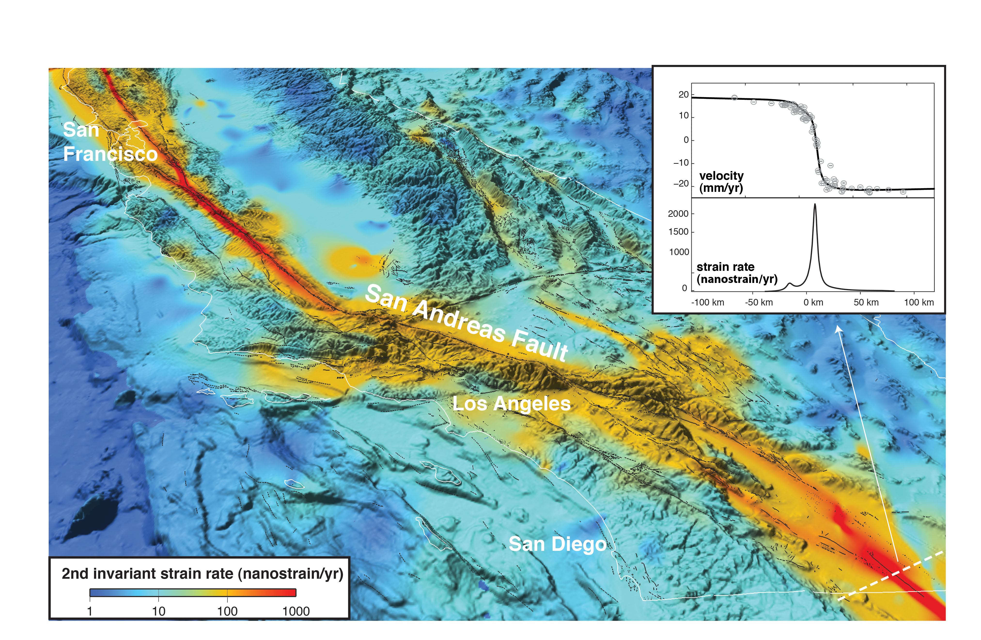
Strain rate, which is typically greatest within 10-50 km of an active fault, is calculated by taking the spatial derivative of measured crustal velocities (Top Figure). Full resolution of velocity gradients requires a spatial sampling at about 1/4 of the typical 6-18 km fault locking depth (Smith and Sandwell, 2003), which is less than the typical ~10 km spacing of the presentday PBO network along the San Andreas system (Wei et al., 2010). A physical model (e.g, McCaffrey, 2005; Meade and Hager, 2005; Smith-Konter and Sandwell, 2009; Bird, 2009) or an interpolation method (e.g., Platt et al., 2007; Freed et al., 2007; Kreemer et al., 2009) must, therefore, be used to compute continuous velocities before obtaining a strain rate map. Simple dislocation models predict that strain rate is proportional to slip rate divided by the locking depth, so even when using similar slip rates, strain rates can differ by a factor of 2-3 because of different fault depth assumptions.
A collaborative effort involving 15 research groups is currently comparing large-scale plate boundary strain rate maps to establish best practices for strain rate estimation (see SCEC UCERF Workshop Report, 2010). Two main conclusions can be drawn from comparing the community maps: 1) Nearly identical GPS datasets result in very different maps, and 2) It is difficult to determine which maps capture the true strain rate best. Maps derived from isotropic interpolation suggest lower rates (e.g., 50-500 nanostrain/year, Imperial fault) than maps generated from dislocation models and methods that localize strain onto faults (e.g., 1000- 2700 nanostrain/year, Imperial fault). The large variations are mainly due to different methods used to construct a high resolution (1 km) map from sparse (~10 km) GPS data. Second order differences can be attributed to assumed fault locations and rheological assumptions.
How can the geodetic community improve accuracy and resolution of strain rate maps? First, when GPS resolution is inadequate, proper localization of strain seems to require that models include major fault locations. Second, a solution is to densify the GPS network such that station spacing is smaller than the spatial variations in crustal strain. This approach has been tested in areas like the Imperial fault, where strain is adequately resolved (Lyons et al., 2002). Indeed, installation of a few dense GPS arrays across poorly-resolved, high-strain-rate faults is feasible and should be pursued. Recently we deployed a second dense GPS array across the Imperial fault to resolve the high strain rate in the highly-populated Mexicali area of Baja California (Figure 2).
A third approach is to utilize InSAR’s spatial coverage and to stack long time interval interferograms to augment GPS derived estimates. We are developing a remove-stack-restore procedure (Wei et al., 2010) to optimally combine GPS and InSAR, which considers signal, measurement noise, sampling rate, and environmental noise characteristics of each system (Figure 3). This method involves constructing a wide-area, 3-D dislocation model from the GPS data; after low-pass filtering at 40 km, the model is removed from each interferogram. Because the residual interseismic signal and noise have different scale dependencies, filtering an interferogram can increase the signal-to-noise ratio by as much as 20%. Multiple interferograms are stacked to reduce atmospheric error. Finally, the complete deformation field is constructed by adding the low-pass filtered model back to the stack of interferograms. Application to a large stack of ERS (European Remote Sensing) interferograms in Southern California demonstrates better than 2 mm/yr accuracy over the wide range of length scales (200 m to 500 km). Extending the method to Northern California, where InSAR coherence is poor at C-band, will require using the longer wavelength L-band data from ALOS.
The likelihood of a major earthquake depends on the accumulated stress, which is roughly equal to strain rate multiplied by the crustal shear modulus and the time since the last major rupture. Strain rate mapping is, therefore, only one component needed to forecast earthquakes; paleoseismic estimates of the timing and slip of recent (~2000 years) major ruptures (e.g., Grant and Lettis, 2002; Weldon et al., 2005) are equally important. It is interesting to note that the last four major earthquakes in Southern California have not occurred on faults with the highest slip rate (Landers, 1992; Northridge, 1994; Hector Mine, 1999; and the recent Sierra El MajorCucapah earthquake [Figure 2]). In addition to resolving high strain rates on the primary faults, it is thus very important to measure the lower rates on subsidiary faults that rupture far less often but have recently produced the most damaging events. GPS and InSAR, when optimally integrated, will be the primary geodetic tools for resolving crustal strain rate in the most critical regions of our active plate boundary.
Figures:
[Top] Figure 1: Strain rate of the San Andreas Fault System from a geodetically constrained analytical model. Deep slip occurs on 41 fault segments where geologic slip rate is applied and locking depth is varied along each fault segment to best fit the GPS data. Dashed white line shows location of inset. Inset: cross-section across the Imperial fault. Top: velocity profile (black line) and GPS data (gray circles). Bottom: strain rate across the Imperial fault.
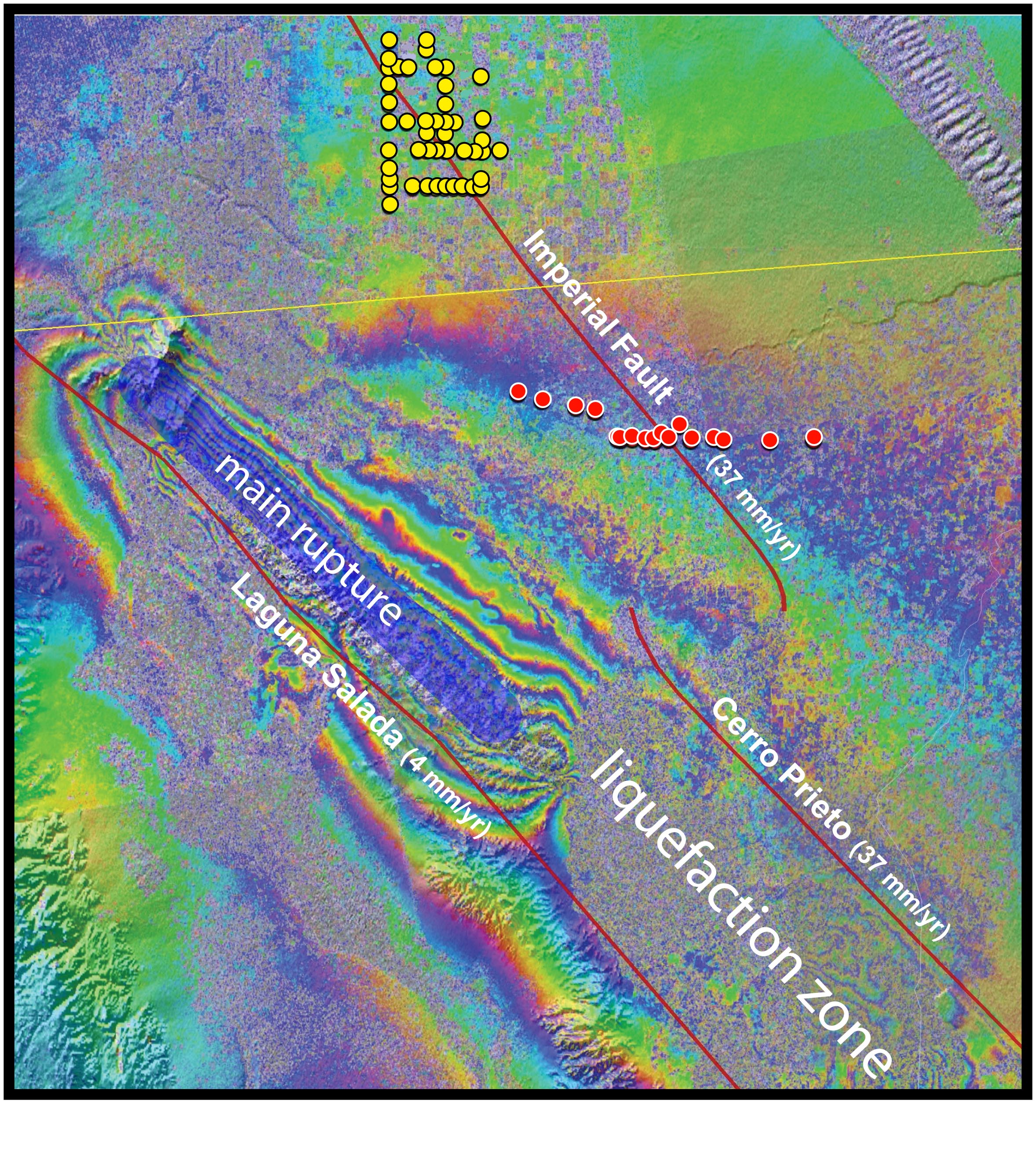
Figure 2: Interferogram of the April 2010 earthquake in Baja California, Mexico, from ALOS PALSAR (Advanced Land Observing Satellite Phased Array type L-band Synthetic Aperture Radar). One color cycle is 11.6 cm of line of sight deformation. Locations of dense GPS monuments across the Imperial fault are also shown. The Imperial array (yellow) was first surveyed in 1993. Reoccupations in 1999, 2000 and 2008 have provided unprecedented accuracy and resolution. In January 2010, 17 new monuments (red) were installed across the fault in Mexicali.

Figure 3: Remove-stack-restore interferograms for the Salton Sea area. (a) Physical model constrained by GPS data. (b) Stacked residual interferograms after applying the filtering method. (c) Final interferogram; sum of (a) and (b). Gray solid lines in (a) and (c) correspond to profile locations in (d). White arrow indicates satellite look direction. (d) Profile across Superstition Hills fault (SHF) and the main faults of the southern San Andreas fault (SAF) system. Arrow identifies short wavelength signal absent in GPS data. (After Wei et al., 2010).
References
Bird, P. (2009), Long-term fault slip rates, distributed deformation rates, and forecast of seismicity in the western United States from joint fitting of community geologic, geodetic, and stress direction data sets, J. Geophys. Res., 114, doi: 10.1029/2009JB006317.
Freed, A. M., S. T. Ali, and R. Bürgmann (2007), Evolution of stress in Southern California for the past 2000 years from coseismic, postseismic and interseismic stress changes, Geophys. J. Int., 169, 1164-1179.
Kreemer, C., G. Blewitt, W. C. Hammond, and H. P. Plang (2009), A high-resolution strain rate tensor model for the western U. S., EarthScope National Meeting 2009, Boise, ID.
Lyons, S. N., Y. Bock, and D. T. Sandwell (2002), Creep along the Imperial fault, southern California, from GPS measurements, J. Geophys. Res., 107, 2249, doi: 10.1029/2001JB000763.
Genrich, J. F., Y. Bock, and R. G. Mason (1997), Crustal deformation across the Imperial Fault: Results from kinematic GPS surveys and trilateration of a densely-spaced, small-aperture network, J. Geophys. Res., 102, 4985– 5004.
Grant. L.B. and W.R. Lettis (2002), Introduction to the special issue on paleoseismology of the San Andreas Fault System, Bull. Seism. Soc. Amer., 92, 2552-2554.
McCaffrey, R. (2005), Block kinematics of the Pacific–North America plate boundary in the southwestern United States from inversion of GPS, seismological, and geologic data, J. Geophys. Res., 110, doi: 10.1029/2004JB003307.
Meade, B. J., and B. H. Hager (2005), Block models of crustal motion in southern California constrained by GPS measurements, J. Geophys. Res., 110, doi: 10.1029/2004JB003209.
Platt, J. P., B. Klaus, and T. W. Becker, The mechanics of continental transforms: An alternative approach with applications to the San Andreas system and the tectonics of California, Earth Plan. Sci. Lett., 274, doi: 10.1016/j.epsl.2008.07.052.
SCEC UCERF workshop report: http://www.scec.org/workshops/2010/gps-ucerf3/Report_ on_2010_SCEC_GPS_UCERF3_Workshop_v2.pdf
Smith, B., and D. T. Sandwell (2003), Coulomb stress along the San Andreas Fault System, J. Geophys. Res, 108, doi:10.1029/2002JB002136.
Smith-Konter, B., and D. T. Sandwell (2009), Stress evolution of the San Andreas Fault System: Recurrence interval versus locking depth, Geophys. Res. Lett., 36, doi: 10.1029/2009GL037235.
Wei, M., D. Sandwell, and B. Smith-Konter (2010), Optimal combination of InSAR and GPS for measuring interseismic crustal deformation, J. Adv. in Space Res., doi: 10.1016/j.asr.2010.03.013
Weldon, R., T. Fumal, G. Biasi, and K. Scharer (2005), Past and future earthquakes on the San Andreas fault, Science, 308, doi: 10.1126/science.1111707.


